Blog

It’s relatively easy to build a model with some data, but part of the expertise involved in a useful piece of analysis is the ability to perform model validation. Model validation gives us a way to tell how useful our model is. Can we trust what it tells us in terms of its predictions and its interpretation?

Model validation encompasses a lot of different techniques, which we can broadly split into two types that have subtly different purposes: in-sample validation and out-of-sample validation.

For ease of explanation, we’re going to use an example to illustrate these concepts. Suppose you are running a marketing campaign which targets members of your customer base with an offer, with the hope that they will go on to make a purchase or subscribe to your service. We have historical data from a similar previous campaign, and we will use this to build a model to predict what is likely to happen with our new campaign. (This is the same example as described in our previous blog on cumulative gains and lift curves.)

In-sample validation

In-sample validation looks at the “goodness of fit”

In-sample validation is concerned with how well the model fits the data that it has been trained on: its “goodness of fit”. Thinking about our example, in-sample validation would help us decide how good our model was for the historic marketing campaign. In-sample validation examines the model fit and is particularly helpful if we are interested in what the current data tell us, e.g., about the relationships between the variables modelled and their effect sizes. By looking at the model coefficients and associated uncertainties of the model we could discover interesting associations, like which types of customer were more likely to respond positively to the campaign (i.e. buy something). In-sample validation will tell us how much trust or confidence we should place in inferences such as this.

One method for in-sample validation is performing a residual analysis. Residuals are an estimate of the error (or noise) in our model and are calculated by taking the difference between the actual outcome values and the outcome values predicted by our model. What we’ll look for in the residuals will be different depending on the type of model being fit. For example, for a linear model we’d expect these to have a normal distribution, that is, some of the residuals to be positive, some negative, centred around zero, and with fewer and fewer residuals as we move further away from zero. If the residuals do not appear to be distributed normally, this may mean that the model’s estimate of the errors shows some systematic trend(s) which in turn implies they are not random, as we would expect in a “valid” model. There are other checks on the model that we could perform as part of in-sample validation, most of which include checking the assumptions upon which the model is built. If the model assumptions aren’t met, this brings into question the validity of any of the findings from the model.

Out-of-sample validation

Out of sample testing refers to using “new” data which is not found in the dataset used to build the model. This is often considered the best method for testing how good the model is for predicting results on unseen new data: its “predictive performance”.

Out-of-sample testing looks at a model’s “predictive performance”

Usually, out of sample testing refers to cross-validation. This is where the model is first built on a subsection of the data – the “training” set – and then tested on the data which was not used to build it – the “test” or “hold-out” set. This gives us a way of looking at how good the model is at predicting results for new data as we can apply the model to what is effectively “unseen” data. Since we are using the hold-out set from the original data we have the advantage of knowing what the true, “real-life” outcome for each datapoint is, meaning we can assess the accuracy of the model by comparing the predicted outcomes to the actual outcomes.

For example, imagine if before we’d run the model on the historical marketing campaign data, we had split off 10% of the data and only run the model on the remaining 90%. We could then use our model to predict whether the remaining 10% of customers would buy the product or not, based on their customer attributes. We could then compare the predictions from our model to the actual outcomes. The closer our predictions are to the actual outcomes for the data, the better our model’s performance for prediction is. For a logistic model (with a binary outcome) such as this, we might be interested in the performance in terms of the sensitivity, specificity and predictive values, calibration, or cumulative gains and lift curves associated with the model.

There are many ways to extend cross-validation beyond taking a single hold-out sample, most of which involve repetition of the method described above in some way or other in order to simulate an increased sample size, reducing variability (i.e., to get a more reliable estimate of the performance). These methods are often applied to machine learning, computationally intensive analysis techniques, where the purpose of the model is to predict or forecast results with great accuracy, with less focus on interpreting the relationships in the data.

Overfitting

An advantage of out-of-sample validation over in-sample validation is that it helps to guard against overfitting. Overfitting is when a model is so specifically tuned to one dataset that the chances of it predicting an accurate outcome for the new data are very small. Figure 1 illustrates this. The left-hand and middle panels show two different models which could be fitted to the data (black points), with the x-axis (horizonal axis) showing the predictor values and the y-axis (vertical axis) showing the outcome values. The blue model (left hand plot) perfectly fits all the data, whereas the green (central plot) model does not accurately predict all the points. The red arrows in the plots below represent the residuals, as discussed above (how far away the model predictons are from the observed data). Comparing these two models in-sample, we can easily see that the blue model is a better fit of the training data.

However, the third plot shows how the different models perform when predicting for new data. The pink cross on this plot represents a new data point with the red arrows pointing to where each model would predict the new outcome to be. This highlights how the blue model is overfit since it would predict the new data much further from its true outcome than the simpler green model. The green model is estimating a more general trend, and is therefore able to predict the new outcome with greater accuracy.

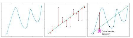
Figure 1: Diagram of modelling 11 data points showing an overfit model (blue) vs a less accurate but more useful model (black). The x-axis (horizontal axis) represents the predictor variables and the y-axis (vertical axis) represents the outcome.

However, there is always a balance between avoiding overfitting and not missing relevant relationships between the variables. This is known as the bias-variance trade-off – a model with high bias is less tied to the training data and oversimplifies the model, whereas a model with high variance is strongly tied to training data and does not generalise well to new data.

One disadvantage of out-of-sample validation is that it reduces the sample size available to fit the model, which is a particular challenge if you only have a small dataset. It is also not necessarily the most appropriate way to test your model if you are not interested in prediction, only interpretation. With our marketing example, if we were only interested in looking at the drivers behind a high chance of making a purchase, we would not be as focused on the predictive power of our model. We would want to trust the underlying assumptions of the model to be confident in interpreting the model’s estimated effects, and so more emphasis would be placed on the in-sample validation, with performing out-of-sample validation taking a back-seat. Though, we may want to consider how well the model performs in different settings. For example, with our marketing model, if we wanted to know how well the model would perform on a different population or at a different time.

Whilst ideally we’d consider all forms of model validation for all models, in practice we may be limited by the data and resources available. Therefore, it’s important to understand the purpose of your model: whether you are more interested in prediction or interpretation. Once you have a good understanding of this, you can use the most appropriate methodology to validate your model focusing on the most relevant assessments, while making the most of the amount of data and other resources you have.