The Importance and Effect of Sample Size
When conducting research about your customers, patients or products it’s usually impossible, or at least impractical, to collect data from all of the people or items that you are interested in. Instead, we take a sample (or subset) of the population of interest and learn what we can from that sample about the population.
There are lots of things that can affect how well our sample reflects the population and therefore how valid and reliable our conclusions will be. In this blog, we introduce some of the key concepts that should be considered when conducting a survey, including confidence levels and margins of error, power and effect sizes. (See the glossary below for some handy definitions of these terms.) Crucially, we’ll see that all of these are affected by how large a sample you take, i.e., the sample size.
Confidence and Margin of Error
Let’s start by considering an example where we simply want to estimate a characteristic of our population, and see the effect that our sample size has on how precise our estimate is.
The size of our sample dictates the amount of information we have and therefore, in part, determines our precision or level of confidence that we have in our sample estimates. An estimate always has an associated level of uncertainty, which depends upon the underlying variability of the data as well as the sample size. The more variable the population, the greater the uncertainty in our estimate. Similarly, the larger the sample size the more information we have and so our uncertainty reduces.
Suppose that we want to estimate the proportion of adults who own a smartphone in the UK. We could take a sample of 100 people and ask them. Note: it’s important to consider how the sample is selected to make sure that it is unbiased and representative of the population – we’ll blog on this topic another time.
The larger the sample size the more information we have and so our uncertainty reduces.
If 59 out of the 100 people own a smartphone, we estimate that the proportion in the UK is 59/100=59%. We can also construct an interval around this point estimate to express our uncertainty in it, i.e., our margin of error. For example, a 95% confidence interval for our estimate based on our sample of size 100 ranges from 49.36% to 68.64% (which can be calculated using our free online calculator). Alternatively, we can express this interval by saying that our estimate is 59% with a margin of error of ±9.64%. This is a 95% confidence interval, which means that there is 95% probability that this interval contains the true proportion. In other words, if we were to collect 100 different samples from the population the true proportion would fall within this interval approximately 95 out of 100 times.
What would happen if we were to increase our sample size by going out and asking more people?
Suppose we ask another 900 people and find that, overall, 590 out of the 1000 people own a smartphone. Our estimate of the prevalence in the whole population is again 590/1000=59%. However, our confidence interval for the estimate has now narrowed considerably to 55.95% to 62.05%, a margin of error of ±3.05% – see Figure 1 below. Because we have more data and therefore more information, our estimate is more precise.
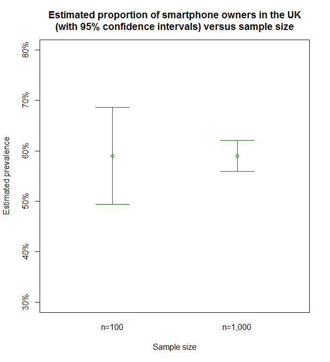
Figure 1
As our sample size increases, the confidence in our estimate increases, our uncertainty decreases and we have greater precision. This is clearly demonstrated by the narrowing of the confidence intervals in the figure above. If we took this to the limit and sampled our whole population of interest then we would obtain the true value that we are trying to estimate – the actual proportion of adults who own a smartphone in the UK and we would have no uncertainty in our estimate.
Power and Effect Size
Increasing our sample size can also give us greater power to detect differences. Suppose in the example above that we were also interested in whether there is a difference in the proportion of men and women who own a smartphone.
We can estimate the sample proportions for men and women separately and then calculate the difference. When we sampled 100 people originally, suppose that these were made up of 50 men and 50 women, 25 and 34 of whom own a smartphone, respectively. So, the proportion of men and women owning smartphones in our sample is 25/50=50% and 34/50=68%, with less men than women owning a smartphone. The difference between these two proportions is known as the observed effect size. In this case, we observe that the gender effect is to reduce the proportion by 18% for men relative to women.
Is this observed effect significant, given such a small sample from the population, or might the proportions for men and women be the same and the observed effect due merely to chance?
We can use a statistical test to investigate this and, in this case, we use what’s known as the ‘Binomial test of equal proportions’ or ‘two proportion z-test‘. We find that there is insufficient evidence to establish a difference between men and women and the result is not considered statistically significant. The probability of observing a gender effect of 18% or more if there were truly no difference between men and women is greater than 5%, i.e., relatively likely and so the data provides no real evidence to suggest that the true proportions of men and women with smartphones are different. This cut-off of 5% is commonly used and is called the “significance level” of the test. It is chosen in advance of performing a test and is the probability of a type I error, i.e., of finding a statistically significant result, given that there is in fact no difference in the population.
What happens if we increase our sample size and include the additional 900 people in our sample?
Suppose that overall these were made up of 500 women and 500 men, 250 and 340 of whom own a smartphone, respectively. We now have estimates of 250/500=50% and 340/500=68% of men and women owning a smartphone. The effect size, i.e., the difference between the proportions, is the same as before (50% – 68% = ‑18%), but crucially we have more data to support this estimate of the difference. Using the statistical test of equal proportions again, we find that the result is statistically significant at the 5% significance level. Increasing our sample size has increased the power that we have to detect the difference in the proportion of men and women that own a smartphone in the UK.
Figure 2 provides a plot indicating the observed proportions of men and women, together with the associated 95% confidence intervals. We can clearly see that as our sample size increases the confidence intervals for our estimates for men and women narrow considerably. With a sample size of only 100, the confidence intervals overlap, offering little evidence to suggest that the proportions for men and women are truly any different. On the other hand, with the larger sample size of 1000 there is a clear gap between the two intervals and strong evidence to suggest that the proportions of men and women really are different.
The Binomial test above is essentially looking at how much these pairs of intervals overlap and if the overlap is small enough then we conclude that there really is a difference. (Note: The data in this blog are only for illustration; see this article for the results of a real survey on smartphone usage from earlier this year.)
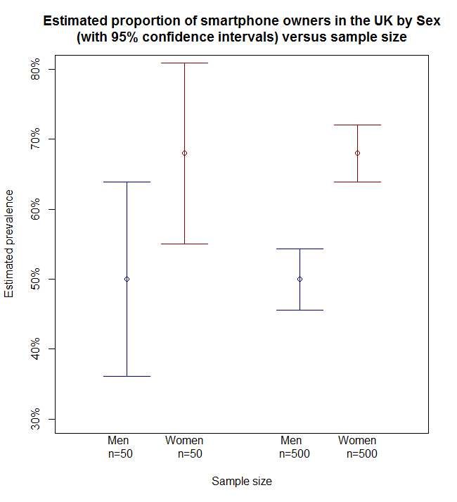
Figure 2
If your effect size is small then you will need a large sample size in order to detect the difference otherwise the effect will be masked by the randomness in your samples. Essentially, any difference will be well within the associated confidence intervals and you won’t be able to detect it. The ability to detect a particular effect size is known as statistical power. More formally, statistical power is the probability of finding a statistically significant result, given that there really is a difference (or effect) in the population. See our recent blog post “Depression in Men ‘Regularly Ignored‘” for another example of the effect of sample size on the likelihood of finding a statistically significant result.
So, larger sample sizes give more reliable results with greater precision and power, but they also cost more time and money. That’s why you should always perform a sample size calculation before conducting a survey to ensure that you have a sufficiently large sample size to be able to draw meaningful conclusions, without wasting resources on sampling more than you really need. We’ve put together some free, online statistical calculators to help you carry out some statistical calculations of your own, including sample size calculations for estimating a proportion and comparing two proportions.
Glossary
Margin of error – This is the level of precision you require. It is the range in which the value that you are trying to measure is estimated to be and is often expressed in percentage points (e.g., ±2%). A narrower margin of error requires a larger sample size.
Confidence level – This conveys the amount of uncertainty associated with an estimate. It is the chance that the confidence interval (margin of error around the estimate) will contain the true value that you are trying to estimate. A higher confidence level requires a larger sample size.
Power – This is the probability that we find statistically significant evidence of a difference between the groups, given that there is a difference in the population. A greater power requires a larger sample size.
Effect size – This is the estimated difference between the groups that we observe in our sample. To detect a difference with a specified power, a smaller effect size will require a larger sample size.
Related Articles
- “Modest” but “statistically significant”…what does that mean? (statsoft.com)
- Legal vs clinical trials: An explanation of sampling errors and sample size (statslife.org.uk)