Blog

In a previous post, we described how a multi-category outcome can be analysed using a multinomial logistic regression model, using the example of programme choice made by US high school students. When fitting the model, we chose to use the “academic” programme as the reference category and thus estimated the changes in the log odds of choosing either a vocation or a general course over an academic course.  We found that the key drivers in the choice of programmes made by students were their socio-economic status, the type of school attended, and their prior reading, maths and science scores.

When fitting a multinomial logistic regression model, one generally wants to understand what motivates the choice made by the student (e.g. what are the key drivers) and how those drivers affect the choice made. For instance, in our example, we might be interested in understanding how the choice of programme varies for students with different maths scores.

Interpreting the model coefficients

As we saw in the model coefficient table in our previous blog, we get two coefficients, one of -0.11 for the comparison between a general and an academic programme and one of -0.14 for the comparison between a vocational and an academic programme. As they are both negative, this tells us that as maths score increases the log-odds of choosing either a general or a vocational programme (instead of an academic programme) decrease. But what does this actually mean? And which programme is actually the most popular choice?

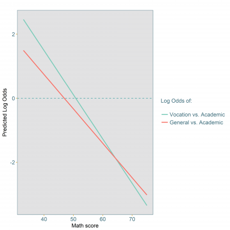
Figure 1: Log-odds of vocational and general choice versus academic choice for student of middle SES and attending public school

To help understand the relationship between maths score and programme choice, we can plot the predictions from the models for a hypothetical student, assuming all other drivers in the model are fixed (i.e. assuming the student is from the middle socio-economic status (SES) group, attends a public school, and has average prior reading and science scores).

In Figure 1, we use the model coefficients to look at the linear relationship (on the log-odds scale) between programme choice and maths score. We can see that, as the maths score increases, the log odds of choosing a vocational vs. academic course are decreasing faster than the log odds of choosing a general vs. academic course, reflecting the difference of size in their model coefficients.

What is interesting from this plot is that for maths scores below 45, both sets of log odds are positive indicating that choosing either of the two programmes is more likely than choosing an academic programme.

We can also see that for a maths score of just above 60 the two lines cross over, i.e. the odds of a general vs. academic choice are now higher than the odds of a vocational vs. academic course.  But what actually are those odds?

What are the odds?

To obtain the odds of either set of choices, we can take the exponential of the predicted log odds above and again plot them against maths score in Figure 2.

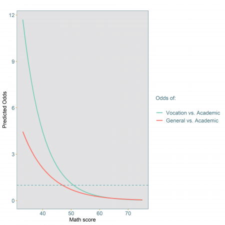
Figure 2: Odds of vocational and general choice versus academic choice for students of middle SES and attending public school

Figure 2 highlights the non-linear nature of the relationships between maths score and the odds of either choices. The difference between the odds is more pronounced for lower values of maths scores with the gap narrowing as maths scores increase. As in the case of a logistic regression, the odds are a measure of the relative association between maths score and programme choice. For example, for a maths score of 40, the odds of choosing a general versus academic programme is 2.1, while the odds of choosing a vocational versus an academic course is 4.4. This means that a student with such a maths score is 2.1 times more likely to choose a general course compared to an academic course, and 4.4 times more likely to choose a vocational course over an academic one.

In addition to what we saw in Figure 1, for maths scores from about 55 upwards both sets of odds are actually quite small, getting close to 0, indicating that both general and vocational courses are very unlikely to be chosen.

Both the odds and log odds plots are useful and accurate representations of the model coefficients. However, they only provide relative measures of the association between maths score and programme choice, using academic programme as the reference for the comparisons. These are thus useful to gain an understanding of the student relative preferences between programmes.

Which courses are student most likely to choose?

At the same time, the model coefficients cannot directly be used to assess which course is most likely to be chosen by an average student attending public school from a middle socio-economic background, as a function of the maths score. To get that information, the odds above needs to be converted to the predicted probability of each outcome (see Figure 3).

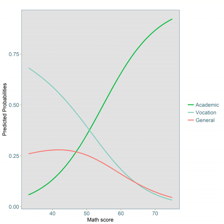
Figure 3: Predicted probabilities of course selection for students of middle SES and attending public school

It is only when the results of the model are converted to probabilities that it becomes obvious that for students with a maths score up to just over 50, a vocational course is more likely to be chosen over any of the other two, while for students with scores higher than that, an academic course is the most likely chosen programme. The other interesting point is that across the whole range of observed maths scores, an average student of middle socio-economic status from a public school is not likely to choose a general course. So regardless of the maths score, middle socio-economic students from public schools with average reading and science scores are unlikely to ever choose a general programme.

As we saw above, the coefficients obtained directly from the model provides an immediate indication as to the direction of the relationships, with the conversion to odds ratio giving an estimate of the relative changes in the odds of choosing one alternative option versus the reference option. However, it is only when converting those odds back to probabilities (as in Figure 3) that one can really see the relationships between the explanatory variables and the likelihood of each outcome.

The output from a multinomial logistic regression model may appear complicated at first and converting the coefficients back to probabilities does make it easier to interpret the model and thus gain useful and actionable insights from it.

In most practical cases, as in the example given here, one is often more interested in how likely each outcome actually is, rather than the relative chance (or odds) of observing one outcome versus another. For instance, a business with a new pricing policy might want to know how sensitive online, in-store or phone customers are to different prices, and might not be so interested in the changes in the balance between online vs. in-store customers, and phone vs. in-store customers as price varies.