Analysing Outcomes with Multiple Categories
In a previous post we described how categorical data can be analysed using generalised linear models. In that blog we focused on binary outcomes, i.e. when you have two possible groups (yes/no, male/female, etc…), and illustrated the approach using the example of modelling the odds of a student being offered a place on a post-graduate course.
Suppose, for example, that instead of modelling the odds of a student being offered a place on a course, we wish to understand the choice a student makes between different types of high-school programmes (e.g. an academic, general or vocational course). Here our response variable is still categorical, but now there are three possible outcomes (academic, general or vocation) rather than two. To explore this, we have data available on the academic choices made by 200 US students. (These data are available from the UCLA Institute for digital research and education using the following link: https://stats.idre.ucla.edu/stat/data/hsbdemo.dta).
In addition to the actual programme choice made by the student, the dataset also contains information on other factors that could potentially influence their choices such as each student’s socio-economic status, the type of school attended (public or private), gender and their prior reading, writing, maths and science scores.
For example, in Figure 1 below we plot the proportion of students that choose each programme by their socio-economic status (classified as low, middle, high). This figure seems to indicate that low income students are less likely to choose an academic programme compared to a general programme. We can also summarise this type of information using contingency tables and a Pearson’s chi-squared test, which are often explored in the initial exploratory analysis of an analysis (see our blog on analysing categorical survey data for more details). For example, a Pearson’s chi-squared confirmed that there is a evidence of a statistically significant association between socio-economic status and degree choice made by the students in our data (p-value = 0.002).
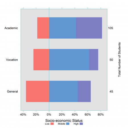
Figure 1: Choice of high-school programme by socio-economic status
While visualisations and simple hypothesis testing are a useful first step to understanding the data, they only look at the effect of one variable in isolation and therefore they do not account for other potential confounding factors such as prior maths or reading scores in this case. Not controlling for confounding factors can lead to incomplete or even wrong conclusions being drawn (for more information see our blog on Simpson’s paradox). We can account for confounding factors by using a more formal approach, in this case a multinomial logistic regression model.
Multinomial Logistic Regression
In a binary logistic regression, we model the probability of the outcome happening (vs. not happening). When extending the approach to model an outcome with multiple categories, we jointly estimate the probabilities of each outcome happening versus a baseline or reference category (usually the most desirable or most common outcome).
While the choice of the reference category does not change the model (i.e. the drivers retained in the model) nor does it change the estimated probabilities of each outcome, it does change how the results are reported. Therefore, the choice of the reference category should be based on the question at hand.
For instance,
- Do we want to understand what motivates high school students to choose vocational or general programmes over an academic course? This could help in understanding the “levers” to improve access to academic programmes or remove barriers to accessing those programmes.
- Or is the emphasis on the vocational course and, therefore, should we use this as the reference category?
Here we choose to use the “academic” programme as the reference category. When we fit the model, we get two sets of model coefficients for each explanatory variable as an output (see Table 1 below), one for each comparison to the reference category. One set estimates the changes in the log odds of choosing a vocational course rather than an academic course and the other of choosing a general course rather than an academic course.
For each variable (and levels of the variable), the table below provides the coefficient estimates for both comparisons of the outcome, along with the standard error and 95% confidence intervals. The p-values reported are for each variable across both comparisons, rather than for the individual comparisons.
| General vs. Academic log odds | Vocational vs. Academic log odds |
|
|||
| Explanatory variable | Coefficient estimate (standard error) | 95% Confidence Interval | Coefficient estimate (standard error) | 95% Confidence Interval | p-value |
| Intercept | -0.29 (0.38) | -1.03; 0.45 | -1.12 (0.46) | -2.03; -0.20 | |
| SES: Middle vs. Low
SES: High vs. Low |
-0.32 (0.49)
-1.04 (0.56) |
-1.28; 0.63
-2.14; 0.07 |
0.86 (0.52)
-0.33 (0.64) |
-0.17; 1.89
-1.60; 0.93 |
0.030 |
| Private vs. Public school | -0.61 (0.55) | -1.68; 0.47 | -2.02 (0.81) | -3.60; -0.43 | 0.012 |
| Reading score | -0.06 (0.03) | -0.11;-0.004 | -0.07 (0.03) | -0.13; -0.01 | 0.027 |
| Maths score | -0.11 (0.03) | -0.17; -0.04 | -0.14 (0.04) | -0.21; -0.07 | < 0.001 |
| Science score | 0.09 (0.03) | 0.03; 0.15 | 0.04 (0.03) | -0.01; 0.10 | 0.004 |
We find that the socio-economic status of students, the type of school, and their prior reading, maths and science scores are all statistically significant for one or both of the comparisons (at the 5% significance level), while there is no evidence that the choice of programme differs between boys and girls (hence why gender is not included in the table).
Note that the p-values reported are for each of the variables in the model across both comparisons. Furthermore, if the confidence intervals for any of the variable do not include zero for a given comparison, this means that this variable has a statistically significant effect on those odds.
It is often (but not always) the case with a multinomial logistic regression, that one variable has a statistically significant effect on the odds for one comparison but not another, i.e. that variable might not be associated with how likely one outcome is compared to the reference, but it could be associated with how likely a different outcome is compared to the same reference.
For example, the coefficients for students attending a private school as opposed to a public school are negative for both the odds of choosing a general vs. an academic programme and a vocational vs. an academic programme, but the coefficient is only statistically significant for the latter. For the comparison between general vs. academic programme, the 95% confidence interval includes 0, meaning that there is no evidence to suggest that a student from a private school (as opposed to a public school) is more or less likely to choose a general programme over an academic. On the contrary there is strong evidence to suggest that a student from a private school (as opposed to public school) is less likely to choose a vocational course over an academic one.
The above example illustrates that rather than interpreting each set of model coefficients uniquely, both sets of coefficients need to be considered in parallel to draw meaningful conclusions.
Whilst the raw model coefficients presented above are useful to understand the general direction of the effects of the different factors, they are not always naturally interpretable because they are reported on the log-odds scale. In a future blog we will discuss the different ways we can present the results of a multinomial logistic regression model such as converting the outputs to odds ratios (using a similar interpretation to the ones presented in our previous blog) or to predicted probabilities. These different outputs allow us to more naturally understand which outcome is more likely to happen or, in our example, which programme is more likely to be chosen by a given student.